
이 글에서 소개하고 있는 소스코드는 사이토 고키가 저술한 “Deep Learning from Scratch”의 첫장에서 소개하고 있는 신경망입니다. 한국어판으로는 한빛미디어의 “밑바닥부터 시작하는 딥러닝2″로도 보실 수 있습니다. 해당 도서의 원저자의 허락 하에 글을 올립니다. 특히 공간상의 좌표와 속성값들에 대한 분류에 대한 내용인지라 GIS 분야에서 흔하게 활용될 수 있는 내용이라고 생각됩니다. 보다 자세한 내용은 해당도서를 추천드립니다.
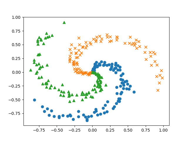
공간 상의 (x,y)에 대한 하나의 지점에 대해서.. 가재, 물방개, 올챙이인 3가지 종류의 식생이 분포하고 있는 생태계가 있다고 합시다. 즉, 입력되는 특성값은 2개일때 3개 중 한개를 결정해야 합니다. 다시 말해, 이미 채집한 데이터가 있고, 이 데이터를 이용해 예측 모델을 훈련시킬 것이며, 훈련된 모델을 이용하면 임이의 (x,y) 위치에 대해 존재하는 식생이 무엇인지를 예측하고자 합니다. 그럼 먼저 예측 모델을 훈련할때 사용할 채집 데이터가 필요한데, 아래의 load_spiral_data 함수가 이러한 채집 데이터를 생성해 줍니다. 아래의 코드는 load_spiral_data 함수를 이용해 채집 데이터를 생성하고 시각화합니다.
import numpy as np
import matplotlib.pyplot as plt

def load_spiral_data(seed=7777):
    np.random.seed(seed)
    DIM = 2  # 입력 데이터 특성 수
    CLS_NUM = 3  # 분류할 클래스 수
    N = 100  # 클래스 하나 당 샘플 데이터 수

    x = np.zeros((N*CLS_NUM, DIM))
    t = np.zeros((N*CLS_NUM, CLS_NUM), dtype=np.int)

    for j in range(CLS_NUM):
        for i in range(N): # N*j, N*(j+1)):
            rate = i / N
            radius = 1.0*rate
            theta = j*4.0 + 4.0*rate + np.random.randn()*0.2

            ix = N*j + i
            x[ix] = np.array([radius*np.sin(theta),
                              radius*np.cos(theta)]).flatten()
            t[ix, j] = 1

    return x, t

x, t = load_spiral_data()
N = 100
CLS_NUM = 3
markers = ['o', 'x', '^']
for i in range(CLS_NUM):
    plt.scatter(x[i*N:(i+1)*N, 0], x[i*N:(i+1)*N, 1], s=40, marker=markers[i])
plt.show()
결과는 아래와 같습니다.
훈련용 데이터가 준비되었으므로, 이제 예측 모델에 대한 신경망에 대한 코드를 살펴보겠습니다. 아래는 은닉층이 1개인 신경망에 대한 클래스입니다. 은닉층이 1개이구요. 이 클래스의 생성자에 대한 인자는 입력되는 특성값의 개수(input_size)와 은닉층의 뉴런 개수(hidden_size) 그리고 분류 결과 개수(output_size)입니다.
class Net:
    def __init__(self, input_size, hidden_size, output_size):
        I, H, O = input_size, hidden_size, output_size

        W1 = 0.01 * np.random.randn(I, H)
        b1 = np.zeros(H)
        W2 = 0.01 * np.random.randn(H, O)
        b2 = np.zeros(O)

        self.layers = [
            Affine(W1, b1),
            Sigmoid(),
            Affine(W2, b2)
        ]
        self.loss_layer = SoftmaxWithLoss()

        self.params, self.grads = [], []
        for layer in self.layers:
            self.params += layer.params
            self.grads += layer.grads

    def predict(self, x):
        for layer in self.layers:
            x = layer.forward(x)
        return x

    def forward(self, x, t):
        score = self.predict(x)
        loss = self.loss_layer.forward(score, t)
        return loss

    def backward(self, dout=1):
        dout = self.loss_layer.backward(dout)
        for layer in reversed(self.layers):
            dout = layer.backward(dout)
        return dout
신경망의 뉴런값과 가중치 그리고 편향에 대한 연산을 위해 Affine 클래스가 사용됬으며, 신경망의 기반이 되는 선형 회귀에 비선형 회귀 특성을 부여하는 활성화함수로 Sigmoid 클래스가 사용되었습니다. 아울러 3개 이상의 출력결과를 확률로 해석하고 이를 기반으로 손실값을 계산할 수 있는 Softmax와 Cross Entropy Error를 하나의 합친 SoftmaxWithLoss 클래스가 사용되었습니다.
먼저 Affine, Sigmoid 클래스의 코드는 다음과 같습니다.
class Affine:
    def __init__(self, W, b):
        self.params = [W, b]
        self.grads = [np.zeros_like(W), np.zeros_like(b)]
        self.x = None

    def forward(self, x):
        W, b = self.params
        out = np.dot(x, W) + b
        self.x = x
        return out

    def backward(self, dout):
        W, b = self.params
        dx = np.dot(dout, W.T)
        dW = np.dot(self.x.T, dout)
        db = np.sum(dout, axis=0)

        self.grads[0][...] = dW
        self.grads[1][...] = db
        return dx

class Sigmoid:
    def __init__(self):
        self.params, self.grads = [], []
        self.out = None

    def forward(self, x):
        out = 1 / (1 + np.exp(-x))
        self.out = out
        return out

    def backward(self, dout):
        dx = dout * (1.0 - self.out) * self.out
        return dx
그리고 SoftmaxWithLoss 클래스는 다음과 같습니다.
class SoftmaxWithLoss:
    def __init__(self):
        self.params, self.grads = [], []
        self.y = None  # Softmax의 출력
        self.t = None  # 정답 레이블

    def forward(self, x, t):
        self.t = t
        self.y = softmax(x)

        # 정답 레이블이 원핫 벡터일 경우 정답의 인덱스로 변환
        if self.t.size == self.y.size:
            self.t = self.t.argmax(axis=1)

        loss = cross_entropy_error(self.y, self.t)
        return loss

    def backward(self, dout=1):
        batch_size = self.t.shape[0]

        dx = self.y.copy()
        dx[np.arange(batch_size), self.t] -= 1
        dx *= dout
        dx = dx / batch_size

        return dx
우의 클래스는 Softmax 연산과 Cross Entropy Error 연산을 각각 softmax와 cross_entropy_error 함수를 통해 처리하고 있습니다. 이 두 함수는 아래와 같습니다.
def softmax(x):
    if x.ndim == 2:
        x = x - x.max(axis=1, keepdims=True)
        x = np.exp(x)
        x /= x.sum(axis=1, keepdims=True)
    elif x.ndim == 1:
        x = x - np.max(x)
        x = np.exp(x) / np.sum(np.exp(x))

    return x

def cross_entropy_error(y, t):
    if y.ndim == 1:
        t = t.reshape(1, t.size)
        y = y.reshape(1, y.size)

    # 정답 데이터가 원핫 벡터일 경우 정답 레이블 인덱스로 변환
    if t.size == y.size:
        t = t.argmax(axis=1)

    batch_size = y.shape[0]

    return -np.sum(np.log(y[np.arange(batch_size), t] + 1e-7)) / batch_size
학습 데이터와 모델까지 준비되었으므로, 이제 실제 학습에 대한 코드를 살펴보겠습니다. 먼저 학습을 위한 하이퍼파라메터 및 모델생성 그리고 기타 변수값들입니다.
# 하이퍼파라미터
max_epoch = 300
batch_size = 30
hidden_size = 10
learning_rate = 1.0

# 모델
model = Net(input_size=2, hidden_size=hidden_size, output_size=3)

# 가중치 최적화를 위한 옵티마이저
optimizer = SGD(lr=learning_rate)

# 학습에 사용하는 변수
data_size = len(x)
max_iters = data_size // batch_size
total_loss = 0
loss_count = 0
loss_list = []
다음은 실제 학습 수행 코드입니다.
for epoch in range(max_epoch):
    # 데이터 뒤섞기
    idx = np.random.permutation(data_size)
    x = x[idx]
    t = t[idx]

    for iters in range(max_iters):
        batch_x = x[iters*batch_size:(iters+1)*batch_size]
        batch_t = t[iters*batch_size:(iters+1)*batch_size]

        # 기울기를 구해 매개변수 갱신
        loss = model.forward(batch_x, batch_t)
        model.backward()
        optimizer.update(model.params, model.grads)

        total_loss += loss
        loss_count += 1

        # 정기적으로 학습 경과 출력
        if (iters+1) % 10 == 0:
            avg_loss = total_loss / loss_count
            print('| 에폭 %d |  반복 %d / %d | 손실 %.2f'
                  % (epoch + 1, iters + 1, max_iters, avg_loss))
            loss_list.append(avg_loss)
            total_loss, loss_count = 0, 0
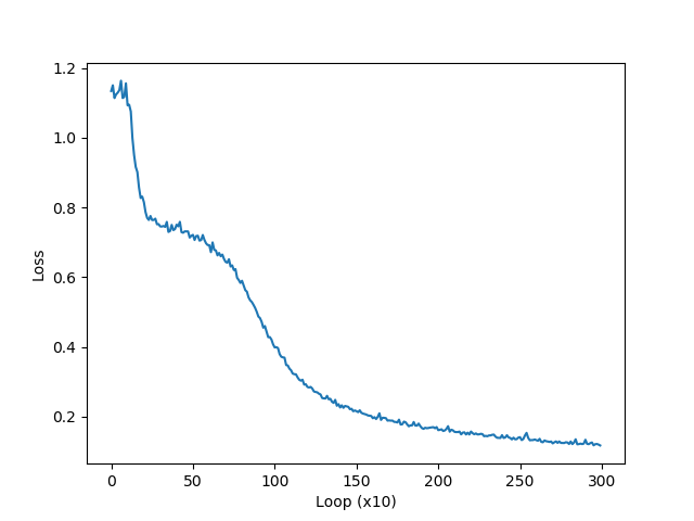
출력값으로써 매 학습 단계마다 손실값이 줄어드는 것을 확인할 수 있습니다.
아래는 위의 학습이 완료되면 그 결과를 시각화해주는 코드입니다.
plt.plot(np.arange(len(loss_list)), loss_list, label='train')
plt.xlabel('Loop (x10)')
plt.ylabel('Loss')
plt.show()
결과는 다음과 같습니다.
이제 이 학습된 모델을 이용해 새로운 입력 데이터를 분류하고 이에 대한 결과를 효과적으로 시각해 주는 코드는 아래와 같습니다.
# 경계 영역 플롯
h = 0.001
x_min, x_max = x[:, 0].min() - .1, x[:, 0].max() + .1
y_min, y_max = x[:, 1].min() - .1, x[:, 1].max() + .1
xx, yy = np.meshgrid(np.arange(x_min, x_max, h), np.arange(y_min, y_max, h))
X = np.c_[xx.ravel(), yy.ravel()]
score = model.predict(X)
predict_cls = np.argmax(score, axis=1)
Z = predict_cls.reshape(xx.shape)
plt.contourf(xx, yy, Z)
plt.axis('off')

# 데이터점 플롯
x, t = load_spiral_data()
N = 100
CLS_NUM = 3
markers = ['o', 'x', '^']
for i in range(CLS_NUM):
    plt.scatter(x[i*N:(i+1)*N, 0], x[i*N:(i+1)*N, 1], s=40, marker=markers[i])
plt.show()
결과는 아래와 같습니다.

![$$loss(x,class)=-\log\biggl(\frac{\exp(x[class])}{\sum_{j}{\exp(x[j])}}\biggr)=-x[class]+\log\biggl(\sum_{j}{\exp(x[j])}}\biggr)$$](http://www.gisdeveloper.co.kr/wp-content/ql-cache/quicklatex.com-f3208d5dfaaecd0f28069ec368ceb1f7_l3.png "Rendered by QuickLaTeX.com")
