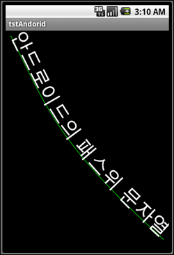
선형 함수에 대한 정의와 그래프 시각화는 다음 코드와 같다.
import numpy as np
import matplotlib.pylab as plt
def identity_func(x):
return x
x = np.arange(-10, 10, 0.01)
plt.plot(x, identity_func(x), linestyle='-', label="identity")
plt.ylim(-10, 10)
plt.legend()
plt.show()
결과는 다음과 같다.

기울기와 y절편을 고려한 선형 함수의 정의는 다음과 같다.
import numpy as np
import matplotlib.pylab as plt
def linear_func(x):
return 2 * x + 1
x = np.arange(-10, 10, 0.01)
plt.plot(x, linear_func(x), linestyle='-', label="linear_func")
plt.ylim(-10, 10)
plt.legend()
plt.show()
결과는 다음과 같다.

계단함수에 대한 정의는 다음과 같다.
import numpy as np
import matplotlib.pylab as plt
def binarystep_func(x):
return (x>=0)*1
x = np.arange(-10, 10, 0.01)
plt.plot(x, binarystep_func(x), linestyle='-', label="binarystep_func")
plt.ylim(-5, 5)
plt.legend()
plt.show()
결과는 다음과 같다.

로지스틱(Logistic) 또는 시그모이드(Sigmoid)라고 불리는 함수 정의는 다음과 같다.
import numpy as np
import matplotlib.pylab as plt
def softstep_func(x):
return 1 / (1 + np.exp(-x))
x = np.arange(-10, 10, 0.01)
plt.plot(x, softstep_func(x), linestyle='-', label="softstep_func")
plt.ylim(0, 1)
plt.legend()
plt.show()
결과는 다음과 같다.

TanH 함수 정의 다음과 같다.
import numpy as np
import matplotlib.pylab as plt
def tanh_func(x):
return np.tanh(x)
x = np.arange(-10, 10, 0.01)
plt.plot(x, tanh_func(x), linestyle='-', label="tanh_func")
plt.ylim(-1, 1)
plt.legend()
plt.show()
그래프는 다음과 같다.

ArcTan 함수 정의는 다음과 같다.
import numpy as np
import matplotlib.pylab as plt
def arctan_func(x):
return np.arctan(x)
x = np.arange(-10, 10, 0.01)
plt.plot(x, arctan_func(x), linestyle='-', label="arctan_func")
plt.ylim(-1.5, 1.5)
plt.legend()
plt.show()
그래프는 다음과 같다.

Soft Sign 함수는 다음과 같다.
import numpy as np
import matplotlib.pylab as plt
def softsign_func(x):
return x / ( 1+ np.abs(x) )
x = np.arange(-10, 10, 0.01)
plt.plot(x, softsign_func(x), linestyle='-', label="softsign_func")
plt.ylim(-1, 1)
plt.legend()
plt.show()
그래프는 다음과 같다.

ReLU(Rectified Linear Unit) 함수는 다음과 같다.
import numpy as np
import matplotlib.pylab as plt
def relu_func(x):
return (x>0)*x
x = np.arange(-10, 10, 0.01)
plt.plot(x, relu_func(x), linestyle='-', label="relu_func")
plt.ylim(-1, 11)
plt.legend()
plt.show()
결과는 다음과 같다.

Leaky ReLU 함수는 다음과 같다.
import numpy as np
import matplotlib.pylab as plt
def leakyrelu_func(x, alpha=0.1):
return (x>=0)*x + (x<0)*alpha*x
x = np.arange(-10, 10, 0.01)
plt.plot(x, leakyrelu_func(x), linestyle='-', label="leakyrelu_func")
plt.ylim(-2, 11)
plt.legend()
plt.show()
결과는 다음과 같다.

ELU(Exponential Linear Unit) 함수는 다음과 같다.
def elu_func(x, alpha=0.9):
return (x>=0)*x + (x<0)*alpha*(np.exp(x)-1)
x = np.arange(-10, 10, 0.01)
plt.plot(x, elu_func(x), linestyle='-', label="elu_func")
plt.ylim(-2, 11)
plt.legend()
plt.show()
결과는 다음과 같다.

TreLU 함수는 다음과 같다.
import numpy as np
import matplotlib.pylab as plt
def trelu_func(x, thres=2):
return (x>thres)*x
x = np.arange(-10, 10, 0.01)
plt.plot(x, trelu_func(x), linestyle='-', label="trelu_func")
plt.ylim(-2, 11)
plt.legend()
plt.show()
결과는 다음과 같다.

SoftPlus 함수는 다음과 같다.
import numpy as np
import matplotlib.pylab as plt
def softplus_func(x):
return np.log( 1 + np.exp(x) )
x = np.arange(-10, 10, 0.01)
plt.plot(x, softplus_func(x), linestyle='-', label="softplus_func")
plt.ylim(-1, 11)
plt.legend()
plt.show()
결과는 다음과 같다.

Bent identity 함수는 다음과 같다.
import numpy as np
import matplotlib.pylab as plt
def bentidentity_func(x):
return (np.sqrt(x*x+1)-1)/2+x
x = np.arange(-10, 10, 0.01)
plt.plot(x, bentidentity_func(x), linestyle='-', label="bentidentity_func")
plt.ylim(-6, 11)
plt.legend()
plt.show()
결과는 다음과 같다.

Gaussian 함수는 다음과 같다.
import numpy as np
import matplotlib.pylab as plt
def gaussian_func(x):
return np.exp(-x*x)
x = np.arange(-10, 10, 0.01)
plt.plot(x, gaussian_func(x), linestyle='-', label="gaussian_func")
plt.ylim(-0.5, 1.5)
plt.legend()
plt.show()
결과는 다음과 같다.
