이미지 분류 모델의 구성 레이어에 대한 결과값 시각화

이미지에 대한 Classification 및 Detection, Segmentation에 대한 신경망 모델을 구성하는 레이어 중 Convolution 관련 레이어의 결과값에 대한 시각화에 대한 내용입니다. 딥러닝 라이브러리 중 PyTorch로 예제를 작성했으며, CNN 모델 중 가장 이해하기 쉬운 VGG를 대상으로 하였습니다.

먼저 필요한 패키지와 미리 학습된 VGG 모델을 불러와 그 레이어 구성을 출력해 봅니다.

import matplotlib.pyplot as plt
from torchvision import transforms
from torchvision import models
from PIL import Image

vgg = models.vgg16(pretrained=True).cuda()
print(vgg)

결과는 다음과 같습니다.

VGG(
(features): Sequential(
(0): Conv2d(3, 64, kernel_size=(3, 3), stride=(1, 1), padding=(1, 1))
(1): ReLU(inplace=True)
(2): Conv2d(64, 64, kernel_size=(3, 3), stride=(1, 1), padding=(1, 1))
(3): ReLU(inplace=True)
(4): MaxPool2d(kernel_size=2, stride=2, padding=0, dilation=1, ceil_mode=False)
(5): Conv2d(64, 128, kernel_size=(3, 3), stride=(1, 1), padding=(1, 1))
(6): ReLU(inplace=True)
(7): Conv2d(128, 128, kernel_size=(3, 3), stride=(1, 1), padding=(1, 1))
(8): ReLU(inplace=True)
(9): MaxPool2d(kernel_size=2, stride=2, padding=0, dilation=1, ceil_mode=False)
(10): Conv2d(128, 256, kernel_size=(3, 3), stride=(1, 1), padding=(1, 1))
(11): ReLU(inplace=True)
(12): Conv2d(256, 256, kernel_size=(3, 3), stride=(1, 1), padding=(1, 1))
(13): ReLU(inplace=True)
(14): Conv2d(256, 256, kernel_size=(3, 3), stride=(1, 1), padding=(1, 1))
(15): ReLU(inplace=True)

.
.

(생략)

위의 특징(Feature)를 추출하는 레이어 중 0번째 레이어의 출력결과를 시각화 합니다. PyTorch는 특정 레이어의 입력 데이터와 그 연산의 결과를 특정 함수로, 연산이 완료되면 전달해 호출해 줍니다. 아래는 이에 대한 클래스입니다.

class LayerResult:
    def __init__(self, payers, layer_index):
        self.hook = payers[layer_index].register_forward_hook(self.hook_fn)
    
    def hook_fn(self, module, input, output):
        self.features = output.cpu().data.numpy()
    
    def unregister_forward_hook(self):
        self.hook.remove()

LayerResult은 레이어의 연산 결과를 검사할 레이어를 특정하는 인자를 생성자의 인자값으로 갖습니다. 해당 레이어의 register_forward_hook 함수를 호출하여 그 결과를 얻어올 함수를 등록합니다. 등록된 함수에서 연산 결과를 시각화하기 위한 데이터 구조로 변환하게 됩니다. 이 클래스를 사용하는 코드는 다음과 같습니다.

result = LayerResult(vgg.features, 0)

img = Image.open('./images/cat.jpg')
img = transforms.ToTensor()(img).unsqueeze(0)
vgg(img.cuda())

activations = result.features

위의 코드의 마지막 라인에서 언급된 activations에 특정 레이어의 결과값이 담겨 있습니다. 이제 이 결과를 출력하는 코드는 다음과 같습니다.

fig, axes = plt.subplots(8,8)
for row in range(8):
    for column in range(8):
        axis = axes[row][column]
        axis.get_xaxis().set_ticks([])
        axis.get_yaxis().set_ticks([])
        axis.imshow(activations[0][row*8+column])

plt.show()

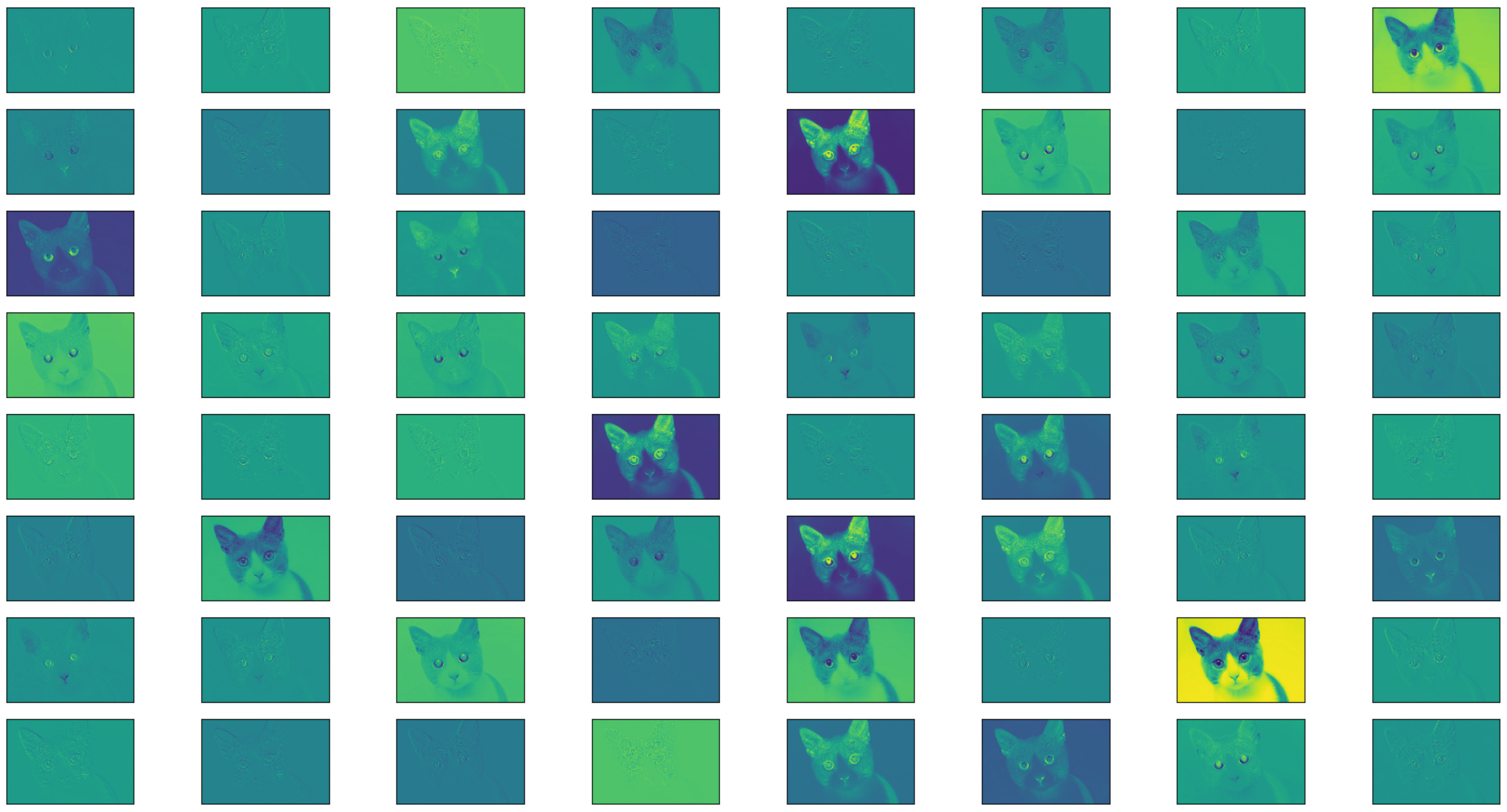
결과 이미지가 총 64인데, 이는 앞서 VGG의 구성 레이어를 살펴보면, 첫번째 레이어의 출력 채널수가 64개이기 때문입니다. 결과는 다음과 같습니다.

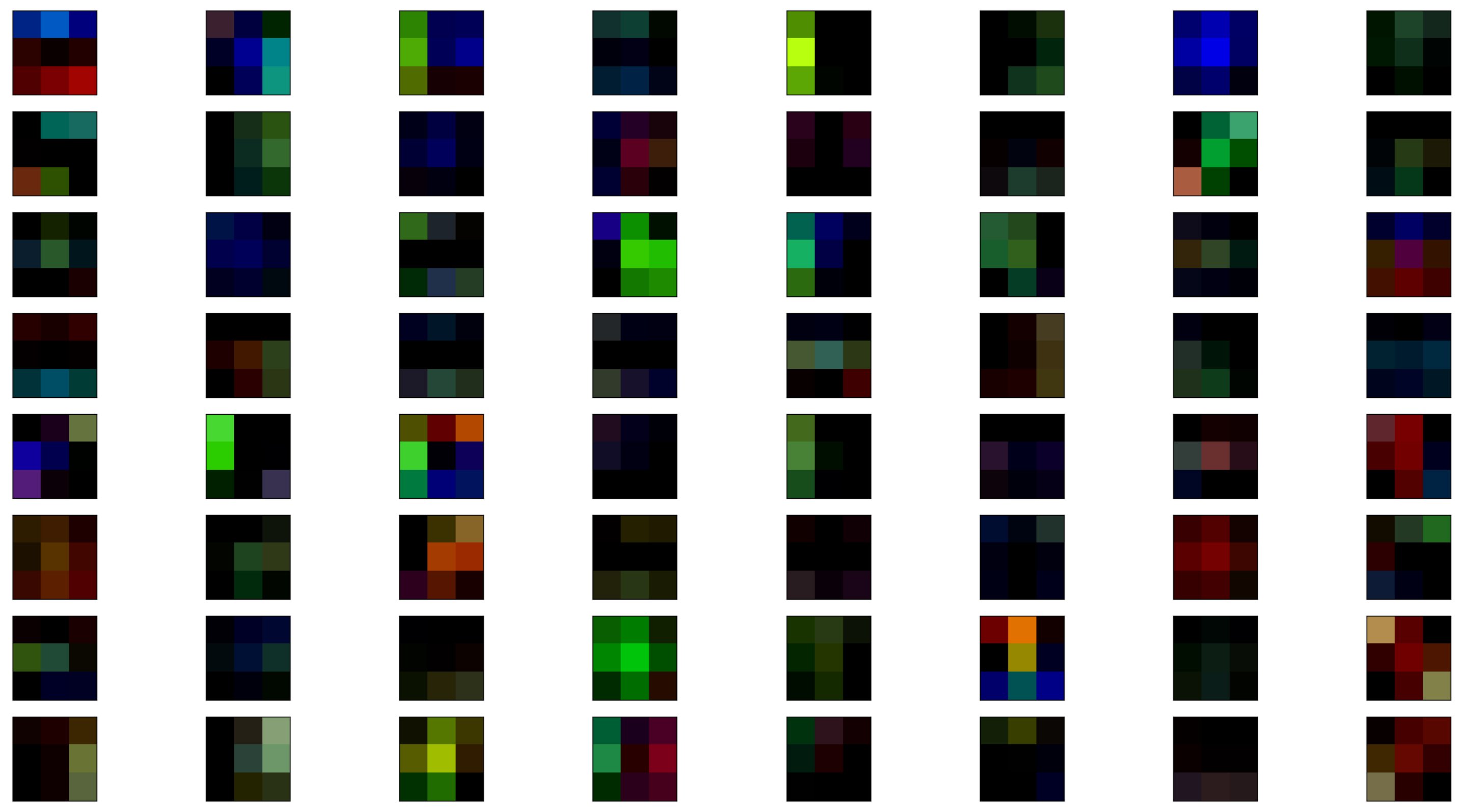
추가로 특정 레이어의 가중치값 역시 시각화가 가능합니다. 아래의 코드가 그 예입니다.

import matplotlib.pyplot as plt
from torchvision import transforms
from torchvision import models
from PIL import Image

vgg = models.vgg16(pretrained=True).cuda()

print(vgg.state_dict().keys())
weights = vgg.state_dict()['features.0.weight'].cpu()

fig, axes = plt.subplots(8,8)
for row in range(8):
    for column in range(8):
        axis = axes[row][column]
        axis.get_xaxis().set_ticks([])
        axis.get_yaxis().set_ticks([])
        axis.imshow(weights[row*8+column])

plt.show()

9번 코드에서 가중치를 가지는 레이어의 ID를 출력해 주는데, 그 결과는 다음과 같습니다.

odict_keys([‘features.0.weight’, ‘features.0.bias’, ‘features.2.weight’, ‘features.2.bias’, ‘features.5.weight’, ‘features.5.bias’, ‘features.7.weight’, ‘features.7.bias’, ‘features.10.weight’, ‘features.10.bias’, ‘features.12.weight’, ‘features.12.bias’, ‘features.14.weight’, ‘features.14.bias’, ‘features.17.weight’, ‘features.17.bias’, ‘features.19.weight’, ‘features.19.bias’, ‘features.21.weight’, ‘features.21.bias’, ‘features.24.weight’, ‘features.24.bias’, ‘features.26.weight’, ‘features.26.bias’, ‘features.28.weight’, ‘features.28.bias’, ‘classifier.0.weight’, ‘classifier.0.bias’, ‘classifier.3.weight’, ‘classifier.3.bias’, ‘classifier.6.weight’, ‘classifier.6.bias’])

위의 레이어 ID로 가중치값을 가져올 레이어를 특정할 수 있는데요. 최종적으로 위의 코드는 다음과 같이 가중치를 시각화해 줍니다.

파이썬의 NLTK 라이브러리를 이용한 WordNet 활용

WordNet은 프린스턴 대학교에서 구축한 유의어 DB인데, 유의어 사이의 관계를 그래프로 정의하고 있는 방대한 데이터입니다. 이 WordNet을 이용하여 유사한 단어를 파악할 수 있고, 각 단어의 유사도를 계산할 수 있습니다. 이를 파이썬의 NLTK를 이용해 활용할 수 있는데, 이에 대한 코드를 정리해 봅니다.

먼저 NLTK 패키지의 설치가 필요합니다. 제 환경에서는 conda install nltk와 같은 식으로 설치하였습니다.

NLTK 패키지의 설치가 끝나면 다음과 같은 코드를 통해 WordNet 데이터를 PC에 다운로드 받을 수 있습니다.

import nltk

nltk.download('wordnet')

가장먼저 ‘man’이라는 단어의 유의어를 검색하기 위해 다음 코드가 사용됩니다.

from nltk.corpus import wordnet

print(wordnet.synsets('man'))
''' Output:
[
    Synset('man.n.01'), 
    Synset('man.n.03'), 
    Synset('man.n.05'), 
    Synset('man.n.06'),     
    Synset('man.n.08'), 
    Synset('man.n.09'), 
    Synset('man.n.10'), 
    Synset('man.v.01'), 
    Synset('man.v.02')],
    Synset('serviceman.n.01'), 
    Synset('homo.n.02'), 
    Synset('valet.n.01'),     
    Synset('world.n.08')
]     
'''

위의 검색에서 man.n.01의 경우 n은 명사를 의미합니다. 참고로 v는 동사이구요. 01은 man에 대한 인덱스값입니다. 이 man.n.01에 대한 사전적 의미를 얻기 위한 코드는 다음과 같습니다.

man = wordnet.synset('man.n.01')
print(man.definition()) # an adult person who is male (as opposed to a woman)

버그인지는 모르겠으나, man.n.02는 검색되지 않았음에도 아래의 코드는 유효합니다.

man2 = wordnet.synset('man.n.02')
print(man2.definition()) # someone who serves in the armed forces; a member of a military force

man.n.01에 대한 단어의 관계 그래프는 다음 코드를 통해 얻을 수 있습니다.

print(man.hypernym_paths())
''' Output:
[
    [Synset('entity.n.01'), Synset('physical_entity.n.01'), Synset('causal_agent.n.01'), Synset('person.n.01'), Synset('adult.n.01'), Synset('man.n.01')], 
    [Synset('entity.n.01'), Synset('physical_entity.n.01'), Synset('object.n.01'), Synset('whole.n.02'), Synset('living_thing.n.01'), Synset('organism.n.01'), Synset('person.n.01'), Synset('adult.n.01'), Synset('man.n.01')], 
    [Synset('entity.n.01'), Synset('physical_entity.n.01'), Synset('causal_agent.n.01'), Synset('person.n.01'), Synset('male.n.02'), Synset('man.n.01')], 
    [Synset('entity.n.01'), Synset('physical_entity.n.01'), Synset('object.n.01'), Synset('whole.n.02'), Synset('living_thing.n.01'), Synset('organism.n.01'), Synset('person.n.01'), Synset('male.n.02'), Synset('man.n.01')]
]
'''

위의 관계 그래프 정보는 총 4개의 list로 구성된 list인데, 이를 시각화하면 다음과 같습니다.

관계 그래프의 경로 역시 4개라는 것을 알 수 있고, 경로의 흐름에 따라 단어의 의미가 점점 구체화됩니다. 이 관계 그래프를 통해 서로 다른 단어에 대한 유사도를 계산할 수 있는데, 아래의 코드가 그 예입니다.

boy = wordnet.synset('boy.n.01')
guy = wordnet.synset('guy.n.01')
girl = wordnet.synset('girl.n.01')
woman = wordnet.synset('woman.n.01')

print(man.path_similarity(man))     # 1.0
print(man.path_similarity(boy))     # 0.3333333333333333
print(man.path_similarity(guy))     # 0.5
print(man.path_similarity(girl))    # 0.25
print(man.path_similarity(woman))   # 0.3333333333333333

단어 간의 유사도는 0부터 1까지의 값으로, 1에 가까울수록 두 단어의 의미가 더욱더 유사하다는 의미이고, 0에 가까울수록 그 의미의 관계가 거의 없다는 것을 의미합니다.