앞서 언급한대로, PropertyGrid에 List 컨트롤을 달아보자. 이 글을 쓰기에 앞서 List 컨트롤을 PropertyGrid에 달아보는 샘플 코드를 작성하면서, 뭐.. “이런 뷁스런”이란 생각이 들었다. 단지 컨트롤 하나 달기 위해 전역 변수이며 새로운 클래스를 2개씩이나 만들어줘야하다니.. .NET에 대한 실망이 쪼끔 인다. 그러나 이 방법말고 좀더 세련된 방법이 있을것이라 생각된다. 한번 시간날때 찾아봐야겠다.
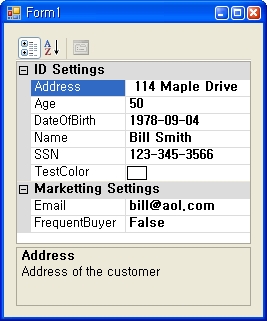
여하튼, 지금 내가 알고 있는 방법을 정리해보자. 먼저 구현할 결과 화면은 다음과 같다.
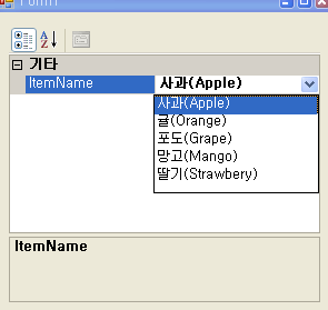 즉, 우리가 추가할 프로퍼티의 이름은 ItemName이고 이 프로퍼티의 값으로 사과, 귤, 포도, 망고, 딸기을 선택할 수 있는 Combo List 컨트롤이라는 도우미를 붙인 형태를 구현하는 방법이다.
먼저 사과, 귤, 포도 등의 문자열들을 담을 string 배열에 대한 전역 변수를 선언한다.
internal class PropertyItemList
{
    internal static string[] _items;
}
비록 PropertyItemList라는 클래스를 전역변수로써 인스턴스화하지는 않겠지만, 맴버변수로 정적으로 선언함으로써 전역변수의 의미를 갖는다. 이렇게 정적으로 선언하여 전역처럼 쓰는 이유는 앞으로 추가할 2개의 새로운 클래스에서 이 PropertyItemList의 _items 정적변수에 접근해야하기 때문이다. 추가할 2개의 새로운 클래스에 대해서 살펴보기 전에 PropertyItemList의 _items 변수에 문자값들을 넣어주는 코드의 살펴보자.
private void Form1_Load(object sender, EventArgs e)
    {
        MyList listItem = new MyList();

        PropertyItemList._items = new String[5];
        PropertyItemList._items[0] = "사과(Apple)";
        PropertyItemList._items[1] = "귤(Orange)";
        PropertyItemList._items[2] = "포도(Grape)";
        PropertyItemList._items[3] = "망고(Mango)";
        PropertyItemList._items[4] = "딸기(Strawbery)";

        propertyGrid1.SelectedObject = listItem;
}
MyList는 앞으로 추가할 2개의 클래스 중 하나이며, propertyGrid의 SelectedObject 속성에 넣어주게 된다. 이는 이미 앞서 살펴봤으므로 이미 잘알고있을것이다.
이제 새로운게 추가할 두개의 클래스를 하나 하나 만들어 보자. 먼저 이미 나와버린 MyList 클래스이다.
public class MyList {
    private string _itemName;

    [Browsable(true)]
    [TypeConverter(typeof(MyConverter))]
    public string ItemName {
        get {
            string S = "";
            if (_itemName != null) {
                S = _itemName;
            } else {
                S = PropertyItemList._items[0];
            }

            return S;
        }

        set { _itemName = value; }
    }
}
ProperrtGrid에 추가할 프러퍼티인 ItemName을 가지고 있으며 Attribute를 지정하고 있다. 여기서 지정된 Attribute에 대해서 살펴보면, Browsable와 TypeConverter이다. Browsable는 원래 지정하지 않아도 되는데, 기본값으로 true이기 때문이다. 의미그대로 PropertyGrid에 나타낼 것이냐 말것이냐를 정하는 것이다. 그리고 TypeConverter가 바로 우리가 추가한 프로퍼티에 리스트 컨트롤을 달게 하는 역활을 하는 Attribute이다. 즉, TyperConverter의 인자로써 어떤 클래스를 주는데, 바로 이 어떤 클래스를 통해 프로퍼티에 리스트 컨트롤을 달거나 프로퍼티를 사용자가 직접값을 수정하게 하거나 리스트 컨트롤에서 선택만 하게 하거나 등의 특성을 지정하는 것이다. 그렇다면 이제 마지막으로 이 어떤 클래스인 MyConverter에 대해 살펴보자.
public class MyConverter : StringConverter
{
    public override bool GetStandardValuesSupported(
        ITypeDescriptorContext context) {
        return true;
    }

    public override bool GetStandardValuesExclusive(
        ITypeDescriptorContext context) {
	return true;
    }

    public override
        System.ComponentModel.TypeConverter.StandardValuesCollection
        GetStandardValues(ITypeDescriptorContext context) {
        return new StandardValuesCollection(PropertyItemList._items);
    }
}
다소, 뷁스러운 클래스라고 생각하는데, 이 하나의 클래스에서 생전보도 못한 .NET 클래스가 참 많이도 나오기 때문이다. 다 집어치우고 필요한 것만 골라 따져보면, 먼저 override한 GetStandardValuesSupported에서 true를 반환해야만 Combo List 컨트롤을 볼수가 있으며 false를 반환하면 우리의 노력은 물거품이 되고 만다. 그리고 GetStandardValuesExclusive라는 매서드의 반환값을 true로 하면 단시 List에서 선택만 할 수 있고 키보드로 문자열값을 변경할 수 없게된다. 마지막으로 GetStandardValues는 List 컨트롤에 나열된 문자열값을 지정해주기 위한 매서드이다.
필자는 “뭔가 잘못된 것 같다”라는 생각이 들었다. 단지 컴보 리스트 컨트롤 하나 추가하기 위한 과정이 이처럼 복잡하다는 이유에서가 아니라, 반드시 전역변수를 선언해야만(여기서는 같은 효과를 위해 정적변수를 선언했다) 한다는 것에서였다. 이 문제는 차츰 해결될 것이라고 생각된다.
끝으로 Blog에 어제부터 google의 AdSense를 달아놨는데.. 이 글이 도움이 되셨다면 댓글말고, 옆에 AdSense 클릭 좀 해주시길~ 댓글은 쓰기 힘드실까봐~ ㅋ –;;